
Month: November 2007
More genes please!
Targeted discovery of novel human exons by comparative genomics:
Here we describe a genome-wide effort, carried out as part of the Mammalian Gene Collection (MGC) project, to identify human genes not yet in the gene catalogs. Our approach was to produce gene predictions by algorithms that rely on comparative sequence data but do not require direct cDNA evidence, then to test predicted novel genes by RT-PCR. We have identified 734 novel gene fragments (NGFs) containing 2188 exons with, at most, weak prior cDNA support. These NGFs correspond to an estimated 563 distinct genes, of which >160 are completely absent from the major gene catalogs, while hundreds of others represent significant extensions of known genes. The NGFs appear to be predominantly protein-coding genes rather than noncoding RNAs, unlike novel transcribed sequences identified by technologies such as tiling arrays and CAGE. They tend to be expressed at low levels and in a tissue-specific manner, and they are enriched for roles in motor activity, cell adhesion, connective tissue, and central nervous system development. Our results demonstrate that many important genes and gene fragments have been missed by traditional approaches to gene discovery but can be identified by their evolutionary signatures using comparative sequence data. However, they suggest that hundreds–not thousands–of protein-coding genes are completely missing from the current gene catalogs.
ScienceDaily makes it intelligible.
One stop linking for personal genomics
The unfortunate consequences of misunderstanding race
Reading the links that come in to GNXP, I happened upon this post on what the author referrs to as “scientific racism”. This bit caught my eye:
I sat on a grant review committee recently for a national-level competition for multi-million dollar grants of an agency I won’t name. The review committee was quite large, probably 25 or more scholars from around the U.S. One of the grant applications that the other reviewers (mostly from the biological sciences) rated the highest was one that proposed to look at the “genetic racial differences among Blacks and whites” to different kinds of treatment for HIV/AIDS. I rated this grant proposal among the lowest I had reviewed because of the methodology: all of the participants in the study would be sorted into the supposedly self-evident categories “Black” and “white” based on self-identification. When I raised this objection among my colleagues in the biological and health sciences, they all blinked hard, and looked at me as if I’d committed some sort of unpleasant faux pas. The chair of the committee finally acquiesced that this was a methodological flaw in the proposal, but the grant was nevertheless awarded millions of dollars.
Biomedical researchers are caught between a rock and a hard place here–none of them enjoy being referred to as scientific racists by their colleagues, I’m sure, but they’re also interested in real phenomena.
It’s well-known that minorities are less likely to participate in biomedical research (though recent studies suggest this is not because they’re less willing). From a geneticist’s perspective, the discomfiting implication of this is that tests of a drug’s efficacy and safety are done on a range of genetic backgrounds that are strongly biased towards the European mean. That is, drugs are accepted or rejected largely based on how well they perform in a sample of individuals of European descent. This is obviously a problem for the applicability of any results, and the NIH is indeed making minority inclusion a requirement for funding certain projects.
Clearly, none of this would be an issue if everyone responded identically to drugs (or if the correlation between drug response and race were zero). It is, however, an issue. Now, ancestry could be related to drug response through any number of mechanisms, either directly (through genetics) or indirectly (through socioeconomic status, etc). Teasing apart those influences means looking at both of them. But then you have someone like the author, who simply dismisses the correlation altogether! And who evidently has some say in the funding of these studies!
It’s worth pointing out that HIV progression does indeed have a genetic component and that certain alleles like CCR5-delta32, which is strongly protective against HIV infection, show marked geographic differences in frequency. A priori, looking for genetic components to differential drug response between populations seems entirely reasonable. Lastly, her main point seems to be that genetic ancestry and self-identified race might not match up. They do.
I’m well-aware that positions like the author’s are made possible by people at the other end of the spectrum, who see races as the embodiment of some Platonic ideal. But rejecting idiocy certainly does not require one to embrace blindness!
Related: Cancer and Race
Brown eyed girl?
Peter Frost states:
I suspect there is some incipient sex-linkage, i.e., European women may be somewhat likelier to have non-brown eyes and non-black hair. If this sex-linkage is mediated by prenatal estrogenization there may also be some impact on personality and temperament. But I really don’t know, and unfortunately there are still more questions than answers.
I’ve read Peter’s book, Fair Women, Dark men, and it is a great collection of data. Also, he has theorized that European color variation is a byproduct of selection selection. So I have been primed to look for a trend where women seem to express blondism or light eye color at higher frequencies. But I just haven’t found anything like that. In fact, I’ve found data which goes in the other direction, that is, females have a higher frequency of brown eyes! But this really clinched it for me:
The source is this paper, Genetic determinants of hair, eye and skin pigmentation in Europeans. Note that women tend to score higher on skin sensitivity toward sun, which implies that they do have ligher skin. And as for hair color, well, perhaps there is a difference in how one judges blonde vs. brunette for males and females? I don’t know. But the eye color data I’ve seen elsewhere and just dismissed it as small N or something like that. At this point my assumption is that there isn’t really the sexual dimorphism in eye color that there is most definitely is in skin color. As for hair, I’m more open to this since it seems that it is subject to more genes, and there could be some hormonal factor as the tendency toward greater blondism in children and females is noted among Australian Aboriginals as well.
Anyway, forget visual inspection. Here’s the associations taking sex into account (from Table 4 of supplementary info):
The authors don’t want to make a judgment based on these data. But I’m not religious about 0.05 P values. And it looks like there’s some action on KITLG anyhow.
Brown out!
 The most common emails I receive are about hair and eye color, and of these the most frequent source seems to be from individuals in interracial relationships. Quite often they are curious as to the possible outcome of their offspring’s phenotype. Sometimes they wonder why their offspring looks the way he or she does. On one disturbing occasion someone was appealing to me to clear up the suspicion of non-paternity because of the unexpected outcome of the offspring’s appearance! Today I received this email:
I have a 19 month old son who is very light skinned, blond hair and blue eyes. My husband (American) is bi-racial. His mother is white and his father is black.
Myself (German), I’m white, same with both of my parents and grandparents. I’m a redhead with greenish brown eyes, my husband has black hair and brown eyes.
What are the odds for this to happen, for us to have a white baby with blond hair and blue eyes?
This question is very common: why does my baby look so white? Succinctly the child’s ancestors are mostly white (American blacks are on average 20% white, so it is likely that the child is more than 75% European in terms of recent ancestors). I’ve offered more detailed expositions on black white twin pairs. The underlying logic is that genetics is discrete, not blending. This is the the insight and power which Mendelian principles introduced to our understanding of evolutionary process. All that being said the above posts and these sorts of jargon-laden assertions really don’t mean much to many people. So I’m going to answer the email above in some more detail below.
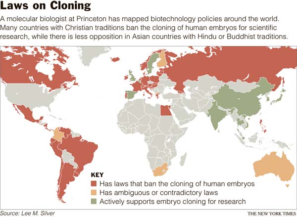
Cloning and culture
An article in The New York Times, Are Scientists Playing God? It Depends on Your Religion, surveys attitudes toward cloning and biological engineering in general. Roughly the thesis being reported is that there is a trichotomy between post-Christian societies, traditional Christian societies and those where Eastern religions predominate. Generally I’m skeptical of these grand cultural typologies, but in this case I think there is an underlying component that explains a large part of the trend: the Roman Catholic Church has long opposed many forms of biological intervention and will no doubt oppose many forms of biological engineering which it deems unethical. Though I do not doubt the sincerity of the believers of the Roman Catholic religion in their adherence to their Church’s position here, I think this is a case where the elite formulation of the clergy and intellectuals has really made a significant impact on public policy. Reading about the anti-abortion movement in the United States during early days after Roe vs. Wade it is clear that the Roman Catholics were at the forefront, and fundamentalist Protestants joined the fray quite a bit later. Similarly, when it came to eugenics laws they were quite widespread in Protestant countries, but the Catholic Church threw up a concerted and consistent resistance to them in nations where it was an institution which could affect public policy significantly.
There are also specific and general problems with the typology. Consider the specific:
Asia offers researchers new labs, fewer restrictions and a different view of divinity and the afterlife. In South Korea, when Hwang Woo Suk reported creating human embryonic stem cells through cloning, he did not apologize for offending religious taboos. He justified cloning by citing his Buddhist belief in recycling life through reincarnation.
When Dr. Hwang’s claim was exposed as a fraud, his research was supported by the head of South Korea’s largest Buddhist order, the Rev. Ji Kwan. The monk said research with embryos was in accord with Buddha’s precepts and urged Korean scientists not to be guided by Western ethics.
Hwang Woo Suk is a convert from Christianity to Buddhism. South Korea is a nation that is about 1/2 non-affiliated, 1/4 Buddhist and 1/4 Christian. Its ethical culture has been traditionally dominated by Confucianism, and there is a powerful substratum of indigenous shamanistic religion which suffuses the practices and outlooks of Christians & Buddhists alike. Christianity is gaining ground among the youth and in the educated segment of the population, and is the dominant religion in Seoul. The last two presidents of South Korea have been Roman Catholic, and that denomination is generally considered the most well educated, affluent and liberal of the religious pillars in South Korean society. South Korea also sends out the most Christian missionaries to the rest of the world aside from the United States. Christian fundamentalists in South Korea have even engaged in iconoclastic violence against Buddhist religious art and statuary. And yet South Koreans were also rather proud of their “cloning research.”
Then there is the biggest general issue with the typology:
By contrast, in the Judeo-Christian tradition, God is the master creator who gives out new souls to each individual human being and gives humans “dominion over soul-less plants and animals. To traditional Christians who consider an embryo to be a human being with a soul, it is wrong for scientists to use cloning to create human embryos or to destroy embryos in the course of research.
I think the term Judeo-Christian is stupid. In any case, not only are there very few Jews in the world, their attitude toward biological engineering tends to be pragmatic and consequentialist from what I can tell. There is one religious group which is left out the typology: Islam. About 15-20% of the world’s population this seems like a large oversight. There don’t seem to be many laws about cloning in the Muslim world, but take a look at abortion laws. Their objection to interventions might be less coherent or precise than those of Roman Catholics, but they seem to mirror them pretty well.
The New York Times piece also points out that in the post-Christian world, such as Sweden, there is a fear of some sorts of biological changes due to a resurgence in a form of natural religion or spirituality. This shouldn’t surprise; the decline of institutional Christianity in northern and eastern Europe has been met with both a rise in a scientific materialist outlook, but even more significantly an unspecified monistic theism reminiscent of pre-Christian traditions. The Left-Right convergences alluded too suggest to me that the typology is too coarse and inchoate. There is a universal “Yuck” within our species, probably rooted in our cognitive hardware. Channeling the impulses culturally can be a tricky thing. For instance, the Japanese and Israelis are far less advanced than Americans in their acceptance or practice of organ donation, generally due to religious rationales. Obviously the Japanese and Israelis don’t share a common spiritual root or background.
Note: I place an emphasis on the Catholic Church as an institution affecting public policy because, for example, abortion rates of Catholics in the United States are at the national average. Moral suasion can only go so far, especially when individuals are making personal utility calculations.
European American population substructure
PLOS early release, Discerning the ancestry of European Americans in genetic association studies:
We have analyzed four different genome-wide data sets involving European American samples, and demonstrated that the same two major axes of variation are consistently present in each data set. The first major axis roughly corresponds to a geographic axis of northwest-southeast European ancestry, with Ashkenazi Jewish samples tending to cluster with southeastern European ancestry; the second major axis largely distinguishes Ashkenazi Jewish ancestry from southeastern European ancestry.
The whole thing is free. Nothing too surprising, just pushing the decimal places further to the right, which is always a good thing when considering something which has medical applications.
Notes on Correlation: Part 2
Part 1 of these notes discussed the general meaning and use of the concepts of correlation and regression. The notes are intended to provide background for other posts I am planning, but if they are of any use as a general introduction to the subject, so much the better.
Part 2 discusses some problems of application and interpretation, such as circumstances that may increase or reduce correlation coefficients. I emphasise that these notes are not aimed at expert statisticians, but at the (possibly mythical) ‘intelligent general reader’. I hope however that even statisticians may find a few points of interest to comment on, for example on the subjects of linearity, and the relative usefulness of correlation and regression techniques. Please politely point out any errors.
Apart from questions of interpretation, this Part contains proofs of some of the key theorems of the subject, such as the fact that a correlation coefficient cannot be greater than 1 or less than -1. There is nothing new in these proofs, but I did promise to give them, and personally I find it frustrating when an author just says ‘it can be proved that…’ without giving a clue how it can be proved. Readers who already know proofs of the main theorems, or are prepared to take them on trust, may prefer to go straight to the section headed ‘Changes of Scale’.
Like Part 1, this Part does not deal with questions of sampling error.
Except for a few passing comments, this Part deals only with bivariate correlation and regression. I am aware that some issues, such as linearity, arise equally (if not more seriously) in the multivariate case. Part 3, if and when I get round to it, will deal with the basics of multivariate correlation and regression.
Notation
These notes avoid using special mathematical symbols, because Greek letters, subscripts, etc, may not be readable in some browsers, or even if they are readable may not be printable. The notation used will be the same as in Part 1, with the following modifications.
In Part 1, the correlation between x and y was denoted by r_xy, the covariance between x and y by cov_xy, the regression coefficient of x on y by b_xy, and the regression coefficient of y on x by b_yx. Since this Part deals only with the correlation of two variables, there will be no ambiguity if the correlation between x and y is denoted simply by r, and their covariance simply by cov. It is necessary to distinguish between the regression of x on y and the regression of y on x, and the coefficients will be denoted by bxy and byx respectively, without the subscript dashes used in Part 1 . These expressions could admittedly be confused with ‘b times x times y’, but I will avoid using the sequences bxy or byx in this sense.
As pointed out in Part 1, for theoretical purposes it is often convenient to assume that variables are expressed as deviations from the mean of the raw values. In this Part the variables x and y will stand for deviation values unless otherwise stated.
As previously, S stands for ‘sum of’, s stands for ‘standard deviation of’, ^2 stands for ‘squared’, and # stands for ‘square root of’.
The derivation of the coefficients
As noted in Part 1, the Pearson regression of x on y is given by the coefficient Sxy/Sy^2, where x and y are deviation values. This is the formula which minimises the sum of the squares of the ‘errors of estimate’, in accordance with the Method of Least Squares. As it is the most fundamental theorem of the subject, it is worth giving a proof, using elementary calculus. (The result can be obtained without explicitly using calculus, but the explanation is then rather longer.)
We want to find a linear equation, of the form x = a + by, such that the sum of the squares of the errors of estimate, S(x – a – by)^2, is minimised.
Provided the x and y values are expressed as deviations from their means, the constant a must be zero. (If we use raw values instead of deviation values, a non-zero constant will usually be required.) The sum of squares S(x – a – by)^2 can be expanded as
Sx^2 + Na^2 + b^2(Sy^2) – 2bSxy – 2aSx + 2abSy. But the last two terms vanish, as with deviation values Sx and Sy are both zero. This leaves Na^2 as the only term involving a, and Na^2 has its lowest value (for real values of a) when a = 0. At its minimum value the expression S(x – a – by)^2 therefore reduces to S(x – by)^2.
It remains to find the value of the coefficient b for which S(x – by)^2 is minimised. This expression may be regarded as a function of b, which may be expanded as:
f(b) = Sx^2 + b^2(Sy^2) – 2bSxy
where Sx^2, Sy^2, and Sxy are quantities determined by the data.
Applying the standard techniques of differentiation, the first derivative of f(b), differentiated with respect to b, is 2bSy^2 – 2Sxy. According to the principles of elementary calculus, if the function has a minimum value, its rate of change (first derivative) at that value will be zero, so to find the minimum (if there is one) we can set the condition 2bSy^2 – 2Sxy = 0. Solving this equation for b, we get b = Sxy/Sy^2 as a unique solution. In principle, this could be a maximum or a stationary point rather than a minimum, but it can be confirmed that for values of b either higher or lower than Sxy/Sy^2 the function f(b) has a higher value. Therefore b = Sxy/Sy^2 gives a unique minimum value for the sum of squares, and may be designated as bxy, the required coefficient of the regression of x on y. The best estimate of x, for a given value of y, is x = (bxy)y.
By similar reasoning we can derive Sxy/Sx^2 as the coefficient of the regression of y on x. The correlation coefficient r can then be derived as the mean proportional between the two regression coefficients, or in the Galtonian manner by ‘rescaling’ the x and y values by dividing them by sx and sy respectively, giving r = Sxy/Nsx.sy.
These formulae use deviation values of x and y. If we prefer to use raw values, the appropriate formulae can be obtained by substitution. Using x and y now to designate raw values, the deviation value of x equals x – M_x, where M_x is the mean of the raw values. Similarly the deviation value of y equals y – M_y. Substituting these expressions for the deviation values of x and y in the above equation x = (bxy)y, we get the formula for raw values x = (bxy)y + M_x – (bxy)M_y. By the same methods we get y = (byx)x + M_y – (byx)M_x. These equations can be represented graphically by straight lines intercepting the axes at points determined by the constants [M_x – (bxy)M_y] and [M_y – (byx)M_x], and with slopes determined by the coefficients bxy and byx.
The range of coefficients
For any positive value of r, expressed in the form Sxy/Nsx.sy, the regression coefficients could range from 0 to infinity, since there is no upper or lower limit on the ratios sx/sy and sy/sx. Similarly, for any negative value of r, the regression coefficients could range from 0 to minus infinity. Unless sx and sy are equal (in which case regression and correlation coincide), one regression coefficient must always be greater and the other less than r. If the regression coefficients are reciprocal to each other (e.g. 2/3 and 3/2), the correlation will be perfect (1 or -1) and there will be a single regression line.
Unlike the regression coefficients, the correlation coefficient r can only range from 1 to – 1. Introductory textbooks often state this without proof, but it is a simple corollary of another fundamental theorem on correlation.
Unless the correlation is perfect (1 or -1), there will be a certain scatter of the observed values of x around the value estimated by the regression of x on y. The coefficient of regressi
on of x on y is Sxy/Sy^2 or r(sx/sy). The estimated values of x for the corresponding values of y are therefore r(sx/sy)y, and the errors of estimate (i.e. the differences between the actual values and the estimated values) will have the form [x – r(sx/sy)y]. But these errors will themselves have a variance, which we may call Ve = [S[x – r(sx/sy)y]^2]/N. [Added: This assumes that the mean value of the errors is zero. Using deviation values of x and y this quite easy to prove, as the mean of the errors is S[x – r(sx/sy)y]/N = (Sx – r(sx/sy)Sy)/N = (0 – 0)/N.] With a little manipulation it can be shown that [S[x – r(sx/sy)y]^2]/N equals (1 – r^2)Vx. [See Note 1.] So we reach the important result that the variance of the errors of estimate of x, as estimated from the regression of x on y, is (1- r^2) times the full variance of x. In other words, the variance of the observed x values around the estimated values is reduced by the proportion r^2 (the square of the correlation coefficient) as compared with the full variance of the x values. It is therefore often said that the correlation of x with y explains or accounts for r^2 of the variance of x. Similarly, it accounts for r^2 of the variance of y. To mark the importance of r^2 it is often known as the coefficient of determination. Since r is a fraction (unless it is 1 or -1), r^2 is smaller than r. The amount of variance explained by r declines more and more rapidly as r itself declines, and a correlation of less than (say) .3 explains very little of the variance. The term ‘explained’ is to be understood purely in the sense just described, and does not necessarily imply a causal explanation.
The estimated values of x themselves have a variance equal to [S[(bxy)y]^2]/N = [S[r(sx/sy)y]^2]/N = [(Sy^2.r^2)Vx/Vy]/N, which can be simplified to (r^2)Vx. Therefore Vx, the total observed variance of x, can be broken down into two additive components, (r^2)Vx + (1 – r^2)Vx, representing the variance of the estimates themselves and the residual variance not accounted for by the correlation.
The closer the correlation (positive or negative), the more of the variance is ‘explained’. If the correlation is perfect (1 or -1) then r^2 = 1 and it ‘explains’ all the variance of x, since there are no errors of estimation at all. If a correlation could be greater than 1 or less than -1, then the variance of the errors, (1- r^2)Vx, would be negative. But a variance cannot be negative, so the correlation coefficient r cannot be greater than 1 or less than -1.
Changes of Scale
The value of the correlation coefficient is unchanged (except sometimes for a reversal of sign) if all the x values, or all the y values, or both, are added to or multiplied by the same constant. For example, if we add a constant k to all the raw x values, then the mean is also increased by k, so the deviation values, the covariance, and the standard deviation, are all unchanged, and therefore the correlation coefficient r = cov/sx.sy itself is unchanged. If instead of adding k we multiply all the raw x values by k, where k is positive, then the mean, the deviation values, and the covariance are also multiplied by k. But so is the standard deviation, so the factor k cancels out of k.cov/k.sx.sy = r, leaving the correlation coefficient itself unaffected. (If k is negative, the sign of r is reversed, since the covariance changes its sign but the standard deviation does not.) Since each such operation of adding and multiplying (in the manner described) leaves r unchanged, they can be repeated any number of times, and in any order, and still leave r unchanged. This can be useful for practical purposes, because it means that if a correlation coefficient is calculated for any convenient set of x and y values, it will still be valid if we add or multiply by k in the way described. Or we might at first be faced with an inconvenient set of values and then convert them to a more manageable set.
It also means that the value of the correlation coefficient is unaffected by a change of scale in one or both variables, for example by measuring in inches instead of centimetres. A further practical implication is that correlation coefficients may be unaffected, or only slightly affected, even by major changes in the population, provided these affect all members of the population in a similar way. For example, the correlation between the heights of fathers and sons may be unchanged even if the sons grow much taller than the fathers, provided the growth is uniform in absolute or proportionate amount. Another possible example is bias in mental tests. It is sometimes supposed that if test results show the same correlation with some external criterion in two different populations, then the test must be ‘unbiased’ with respect to those populations. As it stands, this inference is unjustified, because the correlations would be unchanged if all the test scores in one population were arbitrarily raised (or lowered) by the same amount, which would surely be a form of bias.
The effect of changes of scale on regression is somewhat more complicated. If we always measure the variables in deviation units, relative to their current means, then the regression coefficients will not be affected by adding constants to one or both raw variables, since the deviation values, the covariance, and the standard deviations, are all unchanged, as in the case of correlation. This is not in general true if one or both of the variables are multiplied by constants. For example, if we multiply all of the y values by k, then Sxy, which is the numerator in the Pearson regression formula for bxy, will be multiplied by k, but the denominator, Vy, will be multiplied by k^2, so the regression coefficient as a whole will be divided by k. However, the value of the product (bxy)y will be unchanged, since one factor in the product is multiplied and the other divided by k. With deviation values the predicted value of the dependent variable is therefore not affected by a change of scale in the independent variable alone.
If we use the regression formula for raw values, the matter is further complicated. Adding constants to one or both variables will usually affect the ‘intercept’ of the regression lines with the axes, but not the ‘slope’, whereas multiplying by a constant is likely to affect both slope and intercept.
Linearity
The above derivation of the regression and correlation coefficients assumes that the ‘best estimates’ of x given y, and y given x, can be expressed by equations of the form x = a + by and y = a + bx, which may be graphically represented as straight lines. For this reason they are usually known as coefficients of linear regression and correlation. [See Note 2 for this terminology.]
The question may be asked whether the assumption of linearity is justified, either in general or in any particular case.
If the correlation between the variables is perfect (1 or -1), the regressions will predict the value of the variables without error, and in a graphical representation the points representing the pairs of associated values will all fall exactly on the regression line (which in this case is the same for both variables). Here the description ‘linear regression’ is obviously justified. But perfect correlation is unusual, and more generally there will be some scatter of values around the regression lines. The usual criterion of linearity, adopted from Karl Pearson onwards, is that for each value (or a narrow range of values) of the independent variable, the mean of the associated values of the dependent variable (the associated ‘array’ of values) should fall on the regression line. By this criterion, if the mean values of all arrays fall exactly on the regression line, the regression is perfectly linear.
Linear or approximately linear regression, in this sense, is quite common. Notably, it occurs when the distribution of both variables is
normal or approximately normal. (Strictly, when the bivariate distribution is normal. The distinction would take too long to explain here.) Francis Galton and Karl Pearson confined their original investigations to this case. Udny Yule extended the treatment of correlation and regression beyond this ‘bivariate normal’ case, but he considered that linear regression ‘is more frequent than might be supposed, and in other cases the means of arrays lie so irregularly, owing to the paucity of the observations, that the real nature of the regression curve is not indicated and a straight line will give as good an approximation as a more elaborate curve’.
Statisticians differ in the importance they attach to linearity. Some say that if there is any significant departure from linearity, then the Pearson regression and correlation formulae are invalid and should not be used. They will give an inefficient estimate which leaves larger ‘errors’ than would be possible with a more sophisticated approach. Others take a more relaxed view, saying that if the non-linearity is not extreme, a linear regression is a useful approximation. Any non-zero Pearson regression will ‘explain’ some of the variance in the data, and give a better estimate (on average) than simply taking the mean of the dependent variable. Whether the increase in the ‘errors’ is a serious problem will depend in part on the purposes of the investigation. If the consequence of error in estimation is a large financial cost, or an injustice to individuals, then it is desirable to seek a more accurate formula.
If the departures from linearity are considered too large, alternatives to simple linear regression may be tried. For example a linear regression may still be obtained if we substitute a suitable function of one or both variables in place of the original values. The best known case (and perhaps the only one commonly arising in practice) is where the logarithms of the original values show a linear regression. This can arise if one of the variables grows or declines at a steady rate of ‘compound interest’ in relation to the other.
Alternatively, the researcher may try fitting a curve (such as a polynomial curve of the form x = ay + by^2 + cy^3….) to the data instead of a straight line, the aim being to pass the curve through the means of ‘arrays’ of the dependent variable. But there is no guarantee that any simple curve will give a good fit to the data, or that it will be any more revealing about the underlying relationships of the variables than a straight line. It should also be emphasised that, unlike with linear regression, there will not necessarily be any simple relationship between the regression of x on y and that of y on x. Each non-linear regression curve has to be separately fitted to the data. The regressions of x on y and y on x may be quite different in form.
Having fitted a curve to the data, as a non-linear regression of x on y or y on x, one may calculate how much of the variance in the dependent variable is ‘explained’ by the regression. But in the non-linear case there is no simple formula for this, and it will not in general be the same for both regressions. Although the term ‘non-linear correlation’ is sometimes used, one cannot properly speak of the correlation between two variables in the non-linear case.
In some cases a non-linear regression formula may give a good fit to the data but still be of doubtful value. Especially in the social sciences, departures from linearity may be due to lack of homogeneity in the population, for example differences of age, sex, race, class, etc. The relationship between two variables (e.g. educational achievement and IQ) might be linear within each subgroup, but quantitatively different in each such group. The ‘best fit’ regression line for the whole population would then probably be non-linear, but would depend on the composition of this particular population and have no wider application. Where a population is known to be heterogeneous with respect to the variables of interest, it would be better to disaggregate the data and treat each group separately. Failing that, a straight line regression, which averages out the characteristics of the different groups, may be the most useful single indicator. It is my impression that non-linear regression and correlation are not used much in practice outside the physical sciences, where it is reasonable to expect very precise relationships between variables.
Regression versus correlation?
Regression and correlation are closely related, both mathematically and historically. Some statisticians have however contrasted the roles of regression and correlation, and see one as more useful than the other, or as having different fields of application.
In the time of Karl Pearson and his students the main emphasis was put on the correlation coefficient, which is independent of scale and gives a measure of the extent to which one variable is ‘explained’ by another. A reaction against this emphasis on the correlation coefficient was led by R. A. Fisher, who said: ‘The idea of regression used usually to be introduced in connexion with the theory of correlation, but it is in reality a more general, and a simpler idea; moreover, the regression coefficients are of interest and scientific importance in many classes of data where the correlation coefficient, if used at all, is an artificial concept of no real utility.’ (R. A. Fisher, Statistical Methods for Research Workers, 14th edition, 1970, p.129. The quoted passage goes back to the 1920s.) Cyril Burt remarked that ‘A correlation coefficient is descriptive solely of the set of figures on which it is based: it cannot profess to measure a physical or objective phenomenon, as a regression coefficient or a covariance may under certain conditions claim to do’ (The Factors of the Mind, 1940, p.41). The American statistician John Tukey once joked that he was a member of a ‘society for the suppression of correlation coefficients – whose guiding principle is that most correlation coefficients should never be calculated’. More recently, M. G. Bulmer has said: ‘It is now recognised that regression techniques are more flexible and can answer a wider range of questions than correlation techniques, which are used less frequently than they once were’ (Principles of Statistics, Dover edn., p.209).
This contrast between regression and correlation may seem surprising, as the Pearson coefficients of correlation and regression differ only by a factor of scale, and can be regarded as standardised and unstandardised variants of the same statistic. If we have the information necessary to calculate one of them, we can also calculate the others, since they all involve the covariance of x and y, and the data required for calculating the covariance is sufficient also to determine the coefficients of correlation and regression. But this overlooks the fact that regression coefficients can be estimated from more limited data, without knowing the covariance in the population as a whole. As Fisher pointed out, if we want to know the expected value of x for a given value of y, it is possible to estimate the regression function (whether linear or not) by taking samples of data from a few selected parts of the range of y. Unlike the correlation coefficient, the regression estimate is unaffected by errors in the measurement of x (the dependent variable), provided these go equally in either direction. The correlation coefficient may also vary according to the nature of the sample (such as restriction of range), in ways that do not affect the regression coefficients so strongly. A correlation coefficient cannot be considered ‘objective’ unless it is based on a random or representative sample of the relevant population. However, provided this condition is met, the correlation seems to be just as much an objective characteristic of the population as the regressions. It may be argued that the regression coefficients are less likely to vary dr
amatically in moving from one population to another, but one would wish to see empirical evidence for this in any particular field.
The use made of correlation and regression in practice depends on the field of study. Correlation coefficients are still very widely used in psychometrics, where the scale of measurement is often arbitrary and regression coefficients would vary with the choice of scale. In the social sciences, correlation is probably less widely used, whereas regression analysis (usually multivariate regression) is one of the main instruments of research.
Problems of interpretation
Correlation and regression raise various problems of interpretation, some of which are well known, others less so. To list some of the more important ones:
a) Restriction of range
If the x variable, or the y variable, or both, cover only a limited part of the whole population, the correlation will usually be weakened.
b) Aggregation of data
If a correlation is calculated between data that have been aggregated or averaged in some way, e.g. geographically, the correlations will often be higher – sometimes much higher – than if they were calculated at a less aggregated level.
Points (a) and (b) are both discussed in an earlier post here.
c) Correlation due to pooling of heterogeneous groups
If we have two population groups, which have different means for the x and y variables, then if the data from the two groups are combined there will be a correlation between x and y even if there is no correlation within each population group.
d) Correlation due to mathematical relationships
If one of the variables is actually a part of the other (e.g. length of leg as a part of total height), we will naturally expect there to be a correlation between them. Other mathematical relationships between the variables may also give rise to correlations. For example, if the corresponding x and y values are each arrived at by dividing some data by a third variable, which has the same value for the x and y items in each pair but different values for different pairs, then a correlation will arise (sometimes known as ‘index correlation’) even if the initial data are uncorrelated. Karl Pearson described these as ‘spurious correlations’, but whether they are really to be regarded as spurious depends on the circumstances.
e) Correlation between trends
If the x and y data represent quantities which vary over time, they will often show some long term trend: a tendency (on the whole) either to increase or decrease. If any two such data sets are paired, with the corresponding x and y items in the same chronological order, they will show a correlation: positive if the two trends are in the same direction, negative if they are in opposite directions. Such correlations can be very high. I once constructed two artificial data series, with 20 items of increasing size in each, and deliberately tried not to make the increases too regular, but still found a correlation between the two series of .99! Such correlations can arise regardless of the nature of the data. For example, there would doubtless be a positive correlation between prices in England from 1550 to 1600 and real incomes in Japan from 1950 to 2000 (paired with each other year by year), because there was a rising trend in both. In this case no-one is likely to suppose that there was a causal connection between the two trends, but in other cases there is a real danger. If the two variables are of such a kind that there plausibly may be a causal connection, and they are observed over the same period in the same place, there is a risk that any correlation will be taken more seriously than it should be. For example, if we measure the consumption of pornography and the incidence of rape in the same decade in the same country, there is likely to be some correlation between them. If it is positive, the puritan will say: ‘Aha, pornography causes rape!’. If it is negative, the libertarian will say: ‘Aha, pornography provides a safe outlet for sexual urges!’ Both conclusions are unjustified, because the mere existence of a correlation between two trends, no matter how strong, is almost worthless as evidence of anything. Yule called these ‘nonsense correlations’. He pointed out that in principle a similar problem could arise with geographical trends, such as a north-south gradient, though it was more difficult to find plausible examples. A slightly different case is correlation with wealth or income. Very many traits are correlated with economic prosperity (individual or national), so they are also likely to be correlated with each other. In this case a correlation, even a strong one, between traits is not good evidence of any direct causal connection between them. I would suggest that in the human sciences (psychology, sociology, etc) any very strong correlation (higher than, say, .9) should be viewed with suspicion, and we should examine whether some statistical technicality (such as a grouping effect) is behind it.
f) Correlation and causation
In every textbook the warning is given that ‘correlation does not imply causation’. Up to a point this is correct: the examples of index correlations, and of correlations between trends, show that there may be correlations even when there is nothing that we would properly describe as a causal relationship. Unfortunately the textbooks seldom go on to say that correlation usually does imply a causal connection of some kind, even if it is obscure and indirect. The business of the investigator is then to formulate hypotheses to explain the connection, and to find ways of testing them. Sewall Wright’s path analysis was designed for this purpose. The main problem arising is how to interpret the relations between more than two variables.
g) Regression towards the mean
The concept of regression also involves a danger of fallacies or paradoxes, which I discussed here.
Note 1: We start with the equation
(1) Ve = [S(x – r.y.sx/sy)^2]/N.
Expanding the expression in square brackets we get:
(2) Ve = (Sx^2 – 2Sxy.r.sx/sy + Sy^2.r^2.Vx/Vy)/N.
But Sx^2 = NVx, also Sxy = Nr.sx.sy, and Sy^2 = NVy, so substituting these expressions where appropriate in equation (2) we get:
Ve = (NVx – 2Nr.sx.sy.r.sx/sy + r^2.NVy.Vx/Vy)/N
= (NVx – 2r^2.NVx + r^2.NVx)/N
= (1 – r^2)Vx.
Note 2: Some confusion has arisen about the meaning of the terms ‘linear’ and ‘non-linear’ regression. Traditionally, at least until the 1970s, the term ‘linear regression’ was confined to cases where the regression equation can be represented graphically by a straight line (or by a plane or hyperplane in the multivariate case). For example: ‘If the lines of regression are straight, the regression is said to be linear’ (G. Udny Yule and M. Kendall, Introduction to the Theory of Statistics, 14th edition, 1950, p213), and ‘When the regression line with which we are concerned is straight, or, in other words, when the regression function is linear…. ‘ (R. A. Fisher, Statistical Methods for Research Workers, 14th edition, 1970, p131). Many other examples could be cited. Regression that is not linear in this sense was described as ‘curvilinear’ (Yule, p.213) or ‘non-linear’ (Yule, p.255). More recently some authors have extended the term ‘linear regression‘ to a wider class of functions, including those previously described as ‘curvilinear’. Those who adopt this new usage may even accuse those (probably still the majority) who follow the traditi
onal usage of being in error. One wonders what Fisher would have said.
The genomic future is almost here?
Technology dramatically speeds gene mapping. A short little piece which repeats the standard mantras; faster, cheaper and better. The Human Genome Project was proof of principle. Right now, with all the stuff that is starting to bubble up around personal genomics it looks like we’re at a technological and social point of no return, the second derivative is positive, the the rate of change is increasing. Hsien-Hsien is going to have to start getting a bit more selective about what she blogs about since the sample space of upon which the commentary is based will start to rapidly increase in size.
Though I do have to say stuff like this gets a bit old: